Introduction
Over the last seven articles in this series, we have built up the exposure calculation from the ground up: counterparty credit risk fundamentals, Replacement Cost in full, and then the Adjusted Derivative Contract Amount and Hedging Set Amount for each of the five recognised asset classes — interest rate, exchange rate, equity, credit, and commodity.
This final article closes the loop. We take the five Hedging Set Amounts produced by the asset-class articles, combine them into a single Aggregated Amount, apply the PFE Multiplier, calculate the full Potential Future Exposure, add it to Replacement Cost to get Exposure at Default. This article gives you a clear idea as to what is the SA-CCR: PFE Multiplier and Exposure at Default figures.
To keep this concrete, we carry forward one consistent worked example using figures drawn directly from the worked examples in Parts 2 through 7 of this series, so you can see exactly how the numbers from each individual asset-class article feed into this final calculation.
Step 1 — Recap: What We Already Have
Before going further, let us consolidate what the previous six articles produced for a single hypothetical netting set with one counterparty, drawing on the Hedging Set Amounts calculated in each asset-class worked example:
| Asset Class | Hedging Set Amount (HSA) | Source |
| Interest Rate (USD) | $794,800 | Part 3, Worked Example 3 |
| Exchange Rate (EUR/USD) | $502,588 | Part 4, Worked Example 5 |
| Equity | $8,108,000 | Part 5, Worked Example 4 |
| Credit | $1,031,000 | Part 6, Worked Example 4 |
| Commodity (Energy) | $3,368,000 | Part 7, Worked Example 5 |
We also carry forward the Replacement Cost figure from Part 2, Worked Example 2 (the margined netting set example): RC = $1,500,000.
Step 2 — The Aggregated Amount
The Aggregated Amount, denoted A throughout §217.132, is the foundation input for this calculation. It is simply the sum of every Hedging Set Amount within the netting set, across all asset classes:
| A = Σ (Hedging Set Amounts across all asset classes) |
| Every hedging set in the netting set contributes once — regardless of asset class — to this single aggregated figure. |
| Worked Example 1 — Aggregated Amount Interest Rate HSA: $794,800 Exchange Rate HSA: $502,588 Equity HSA: $8,108,000 Credit HSA: $1,031,000 Commodity HSA: $3,368,000 A = 794,800 + 502,588 + 8,108,000 + 1,031,000 + 3,368,000 A = $13,804,388 |
Notice how dominant the equity exposure is in this combined figure — over half of the total Aggregated Amount. This is a direct consequence of equity’s comparatively high Supervisory Factor (32% for single-name) relative to interest rate’s flat 0.50%. A bank reviewing this output would immediately recognise that the equity book is the primary driver of this counterparty’s potential future exposure, and risk management attention should be weighted accordingly.
Step 3 — The PFE Multiplier
The PFE Multiplier is the mechanism through which this framework rewards over-collateralisation. Recall the formula introduced in Part 1 of this series:
| Multiplier = min{ 1 ; 0.05 + 0.95 × e^((V−C)/(1.9×A)) } |
| V = fair value of the netting set | C = net collateral held | A = Aggregated Amount from Step 2 |
Three properties of this formula are worth understanding clearly before applying it:
- When V − C is large and positive (the bank has substantial uncollateralised exposure), the exponential term approaches 1, and the multiplier approaches its ceiling of 1.0 — no reduction is given.
- When V − C is negative or small (the netting set is well collateralised, possibly even over-collateralised), the exponential term shrinks toward zero, and the multiplier falls toward its floor of 0.05 — a 95% reduction in recognised PFE.
- The multiplier can never fall below 5%, no matter how much collateral is posted. Some residual potential future exposure is always recognised, reflecting the risk that collateral itself could be insufficient or could fail to be called in time during a fast-moving default.
| Worked Example 2 — Calculating the PFE Multiplier Portfolio fair value across the full netting set (V): $9,000,000 (using the same V as Part 2, Worked Example 2) Collateral held (C): $7,500,000 Aggregated Amount (A, from Step 2): $13,804,388 V – C = 9,000,000 – 7,500,000 = $1,500,000 Exponent = (V-C) / (1.9 × A) Exponent = 1,500,000 / (1.9 × 13,804,388) Exponent = 1,500,000 / 26,228,337 Exponent = 0.0572 e^0.0572 ≈ 1.0588 Multiplier = min{1 ; 0.05 + 0.95 × 1.0588} Multiplier = min{1 ; 0.05 + 1.0059} Multiplier = min{1 ; 1.0559} Multiplier = 1.000 (capped at the ceiling) Because V-C is positive and large relative to A, the multiplier hits its ceiling of 1.0 — no diversification or collateral credit is applied to PFE in this scenario. |
This result is worth pausing on. Even though the netting set holds $7.5 million of collateral against a $9 million portfolio, the multiplier still came out at its maximum value of 1.0. This happens because the formula compares V−C against the Aggregated Amount A, not against V alone. With A at $13.8 million, even a $1.5 million net exposure (V−C) is large enough relative to A to push the exponent close to zero reduction. The multiplier only meaningfully compresses below 1.0 when collateral approaches or exceeds the full portfolio value, driving V−C toward zero or negative.
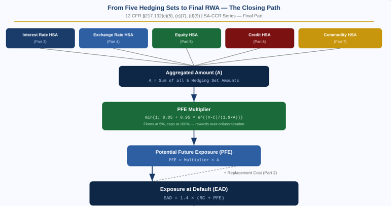
Figure 1: From five Hedging Set Amounts to EAD
Step 4 — Calculating Potential Future Exposure
With the Multiplier and Aggregated Amount both in hand, PFE follows directly:
| PFE = Multiplier × A |
| This is the full potential future exposure across every asset class in the netting set, combined into one figure. |
| Worked Example 3 — Potential Future Exposure Multiplier (from Step 3): 1.000 Aggregated Amount A (from Step 2): $13,804,388 PFE = 1.000 × 13,804,388 PFE = $13,804,388 Since the multiplier hit its ceiling, PFE equals the full Aggregated Amount with no reduction applied. |
Step 5 — Calculating the Final Exposure at Default (EAD)
This is the formula we first introduced all the way back in Part 1 of this series, and everything since has been building toward calculating its two components in full:
| EAD = 1.4 × (RC + PFE) |
| 1.4 is the regulatory alpha multiplier — a conservative buffer applied to the sum of current and potential future exposure. |
| Worked Example 4 — Exposure at Default Replacement Cost (RC, from Part 2, Worked Example 2): $1,500,000 Potential Future Exposure (PFE, from Step 4): $13,804,388 RC + PFE = 1,500,000 + 13,804,388 = $15,304,388 EAD = 1.4 × 15,304,388 EAD = $21,426,143 |
This single number — just over $21.4 million — is the regulatory measure of how much this bank could lose if this specific counterparty defaulted, across every derivative position in the netting set, spanning all five asset classes, accounting for current mark-to-market exposure, potential future market movements, existing collateral, and a conservative regulatory buffer. It compresses an enormous amount of portfolio complexity into one figure that flows directly into the bank’s capital requirement calculation.
Putting the Entire Series Together
It is worth stepping back and seeing the full path from a single derivative trade to a final capital number, drawing on every article in this series:
| Stage | What Happens | Covered In |
| 1. Trade inputs | Notional, maturity, reference entity, credit quality, etc. | Parts 3–7 |
| 2. Adjusted Notional | Notional scaled by duration (IR, Credit) or fair value (FX, Equity, Commodity) | Parts 3–7 |
| 3. ADCA | Adjusted Notional × Delta × Maturity Factor × Supervisory Factor | Parts 3–7 |
| 4. Hedging Set Amount | ADCAs combined within time buckets, reference entities, or commodity types | Parts 3–7 |
| 5. Aggregated Amount (A) | Sum of all Hedging Set Amounts across asset classes | This article |
| 6. PFE Multiplier | Collateral-sensitive scaling factor, floored at 5%, capped at 100% | This article |
| 7. PFE | Multiplier × Aggregated Amount | This article |
| 8. Replacement Cost | Current exposure, margined or unmargined | Part 2 |
| 9. EAD | 1.4 × (RC + PFE) | This article |
Every single one of these ten stages traces back to specific paragraphs within 12 CFR §217.132 — a regulation that, taken as a whole, converts the seemingly abstract question of “how risky is this derivatives counterparty” into a precise, auditable, and replicable dollar figure that determines how much capital a bank must hold.
Quick Summary
- The Aggregated Amount (A) is the sum of every Hedging Set Amount across all five asset classes within a netting set.
- The PFE Multiplier compares net exposure (V−C) against A, rewarding over-collateralisation with a multiplier as low as 5%, but never recognising full collateral protection — some residual PFE is always assumed.
- PFE = Multiplier × Aggregated Amount.
- EAD = 1.4 × (Replacement Cost + PFE) — bringing together the current exposure calculation from Part 2 with the potential future exposure calculation built up across Parts 3 through 7 and this article.
- Banks using the internal models methodology must calculate both stressed and unstressed versions of this entire pipeline and use whichever produces the higher capital requirement.
Frequently Asked Questions
Why did the PFE Multiplier hit its ceiling of 1.0 even with significant collateral posted?
The Multiplier formula compares net exposure (V−C) against the Aggregated Amount (A), not against the gross portfolio value (V) alone. When A is large — as it was in our example, driven heavily by the equity Hedging Set Amount — even a substantial collateral position can leave V−C large relative to A, keeping the exponential term close to its maximum and the Multiplier near 1.0. Meaningful Multiplier compression generally requires collateral that brings V−C close to zero or negative relative to the scale of A.
What is the difference between the Aggregated Amount and the Hedging Set Amount?
A Hedging Set Amount is calculated separately for each asset class (and, for interest rate and exchange rate, separately per currency or currency pair) using that asset class’s specific formula from Parts 3 through 7. The Aggregated Amount is simply the sum of all those individual Hedging Set Amounts across every asset class present in the netting set — it is the single combined figure that feeds into the PFE Multiplier formula.
Why is EAD multiplied by 1.4?
The 1.4 multiplier, called alpha, is a conservative regulatory buffer applied to the sum of Replacement Cost and PFE. It reflects empirical findings that simplified exposure models tend to understate true counterparty exposure, particularly around the tails of the distribution. Banks may apply to use their own estimated alpha, subject to a regulatory floor of 1.2, but the default standardised value is 1.4.
Does a higher EAD always mean a higher capital requirement?
Generally yes, since EAD is a direct multiplicative input into the capital formula K = f(PD, LGD, M) × EAD. However, the counterparty’s PD and LGD matter just as much. A very high EAD against an extremely low-PD, low-LGD counterparty (for example, a well-capitalised sovereign) can still produce a modest capital requirement, while a much smaller EAD against a high-PD, high-LGD counterparty can produce a disproportionately larger one.
What happens differently for banks that don’t use the internal models methodology?
Banks using the standardised approach for counterparty credit risk EAD (the methodology covered throughout this entire series) calculate EAD as shown here and feed it directly into the risk-based capital formula, without the separate stressed/unstressed recalibration that internal-models-methodology banks must perform. The standardised methodology trades away some of that additional risk-sensitivity for a simpler, more auditable, and more consistently comparable calculation across institutions — which is precisely why regulators introduced SA-CCR as the default standardised approach in the first place.