Part A covered the FRTB SBM’s vocabulary, which instruments face which risk charges, and the complete delta and vega formula. This part finishes the job: the curvature formula — genuinely the most intricate piece of MAR21 — and the three correlation scenarios that take the separate delta, vega and curvature numbers and turn them into one final Sensitivities-Based Method capital requirement.
The Idea Behind Curvature Risk
For each risk class, calculating curvature risk means applying an upward shock and a downward shock to each prescribed risk factor, then calculating the incremental loss — for instruments sensitive to that risk factor — above and beyond what the delta risk capital requirement already captures. The size of each shock is itself a risk weight, defined later in MAR21.98 and MAR21.99, which we cover in full in Article 17.
| The Source Document’s Own GIRR Example For GIRR specifically: all tenors of all the risk-free interest rate curves within a given currency — three-month Euribor, six-month Euribor, one-year Euribor, and so on for the euro — must be shifted upward together, applying the prescribed risk weight. The resulting potential loss for each instrument, after deducting the delta risk position, is the outcome of the upward scenario. The same approach is then repeated for a downward scenario. Where an instrument’s price depends on several different risk factors, curvature risk must be determined separately for each one. |
Sourced from MAR21.5(1).
https://www.bis.org/basel_framework/chapter/MAR/21.htm?inforce=20230101&published=20260323
The Curvature Formula, Risk Factor by Risk Factor
The net curvature risk capital requirement for a given risk factor k is captured by two values — an upward version and a downward version — that together measure the aggregate incremental loss beyond the delta capital requirement, for the prescribed shocks. Before the formula itself, here is what each symbol means:
| Symbol | Meaning |
| i | An instrument subject to curvature risk associated with risk factor k. |
| x_k | The current level of risk factor k. |
| V_i(x_k) | The price of instrument i at the current level of risk factor k. |
| V_i(x_k^shock+) and V_i(x_k^shock−) | The price of instrument i after x_k is shocked upward and downward respectively. |
| RW_k^(curvature) | The risk weight for curvature risk factor k, for instrument i. |
| s_ik | The delta sensitivity of instrument i with respect to the delta risk factor that corresponds to curvature risk factor k. |
That last variable, sik, is defined slightly differently depending on the risk class: for the FX and equity risk classes, sik is simply the delta sensitivity of instrument i. For the GIRR, CSR and commodity risk classes, sik is instead the sum of delta sensitivities to all tenors of the relevant curve of instrument i, with respect to that curvature risk factor.


| The Plain-English Version Each formula compares two things: the actual change in an instrument’s price after a shock, versus the change delta alone would have predicted for that same shock (the RWk × sik term). The gap between the two is the curvature loss delta misses — exactly the nonlinear risk we discussed in Part A, where an option’s payoff bends rather than moving in a straight line. One version of the formula captures this gap for the upward shock, the other for the downward shock. |
Sourced from MAR21.5(2), including all sub-points and both formulas, in full.
Within-Bucket Aggregation for Curvature
The curvature risk exposure must be aggregated within each bucket using a prescribed correlation, ρkl, between risk factors k and l. The bucket-level capital requirement, Kb, is defined as whichever is greater: the capital requirement under the upward scenario (Kb+) or under the downward scenario (Kb−).
- Where Kb = Kb+, this is termed “selecting the upward scenario.”
- Where Kb = Kb−, this is termed “selecting the downward scenario.”
- In the specific case where Kb+ equals Kb− exactly, the tie is broken by comparing the sum of all CVRk+ values against the sum of all CVRk− values within the bucket — whichever sum is larger determines which scenario is deemed selected.
One detail worth flagging before we go further: which scenario gets selected — upward or downward — is not necessarily the same across the high, medium and low correlation scenarios we cover later in this article. A bucket could select the upward scenario under one correlation assumption and the downward scenario under another.
The formula also introduces a function, ψ(CVRk, CVRl), which takes the value 0 if CVRk and CVRl both carry a negative sign, and the value 1 otherwise:
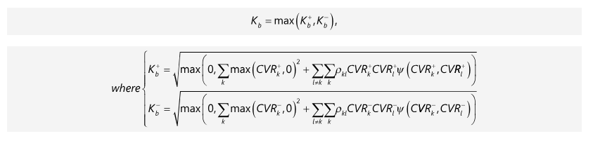
Sourced from MAR21.5(3), including all sub-points and formulas, in full.
Across-Bucket Aggregation for Curvature
Curvature risk positions are then aggregated across buckets within each risk class, using the prescribed correlation γbc between bucket b and bucket c. Sb is defined using whichever scenario (upward or downward) was selected for bucket b in the within-bucket step above — the sum of CVRk+ values if the upward scenario was selected, or the sum of CVRk− values otherwise. A second function, ψ(Sb, Sc), again takes the value 0 if Sb and Sc both carry a negative sign, and the value 1 otherwise.

Sourced from MAR21.5(4), including all sub-points and the formula, in full.
https://www.bis.org/basel_framework/chapter/MAR/21.htm?inforce=20230101&published=20260323
The Three Correlation Scenarios
This is the mechanism that ties the entire SBM together, and it applies uniformly to delta, vega and curvature alike. The Committee’s stated reason for it: correlations between risk factors do not stay stable — they can increase or decrease sharply during periods of financial stress. To address that risk, the full aggregation process from MAR21.4 and MAR21.5 — everything covered in this article and Part A — must be repeated three times over, each time using a different set of values for the correlation parameters ρkl (within a bucket) and γbc (across buckets).
| Scenario | How the Correlation Parameters Are Set |
| Medium correlations | The correlation parameters ρkl and γbc are used exactly as specified in MAR21.39 through MAR21.101 — the risk-class-specific tables we build out in Articles 9 through 17. |
| High correlations | Every ρkl and γbc value is uniformly multiplied by 1.25, subject to a cap at 100%. |
| Low correlations | Every ρkl and γbc value is replaced using the formula below. |


| What the Low-Correlation Formula Is Actually Doing This formula takes whichever of two possible reductions is larger, which keeps the transformation well-behaved across the whole range of possible correlation values. For a high starting correlation (say 90%), doubling and subtracting 100% (2×90%−100%=80%) gives a smaller cut than 75% of the original (67.5%) — so the formula picks 80%, a relatively gentle reduction. For a low starting correlation (say 20%), the same doubling calculation (2×20%−100%=−60%) would be a very aggressive cut, so the formula instead picks 75% of the original (15%), a much gentler reduction. The “greater of the two” rule stops the low-correlation scenario from producing unrealistically extreme or even deeply negative correlations at the low end of the scale, while still meaningfully stressing correlations at the high end. |
Sourced from MAR21.6, including sub-points (1) through (3), in full.
https://www.bis.org/basel_framework/chapter/MAR/21.htm?inforce=20230101&published=20260323
Combining Everything Into the Final SBM Capital Requirement
With three full sets of delta, vega and curvature numbers now calculated — one set per correlation scenario — the last step is genuinely simple, in two parts.
- Step 1: for each of the three correlation scenarios, the bank simply sums up the separately calculated delta, vega and curvature capital requirements, across all seven risk classes, to get one overall capital requirement figure for that scenario.
- Step 2: the Sensitivities-Based Method capital requirement is the largest of the three scenario totals — not an average, and not the medium scenario by default. Whichever scenario produces the biggest number is the one that counts.
This maximum-of-three-scenarios rule is applied in two distinct contexts, both of which we introduced back in Article 5B:
| Context | How the Maximum Rule Applies |
| All instruments across all trading desks | Used for the standard Standardised Approach calculation under MAR11.8(1), MAR20.2, and MAR33.40 — the capital requirement is calculated across every instrument, in every trading desk, combined. |
| Each trading desk on a standalone basis | Used for the per-desk calculation under MAR11.8(2) for Internal Models Approach-eligible desks — capital requirements under each of the three correlation scenarios are calculated and compared separately for every trading desk, with the maximum taken independently at each desk level. |
| Why This Connects Back to Article 5B Recall from Article 5B that IMA banks must calculate the Standardised Approach twice: once across all instruments and desks combined, and separately as a standalone figure for every IMA-eligible desk, with no cross-desk offsetting. MAR21.7 is where that requirement actually gets implemented at the formula level — the three-scenario maximum is taken once for the whole-portfolio calculation, and taken again, independently, for each individual desk. |
Sourced from MAR21.7, including sub-points (1) and (2), in full.
https://www.bis.org/basel_framework/chapter/MAR/21.htm?inforce=20230101&published=20260323
Looking Ahead
This completes our coverage of MAR21.1 through MAR21.7 — the general provisions and the full delta, vega and curvature formulas. Every risk-class article from here forward (Articles 9 through 17) is simply supplying the risk factor definitions, sensitivity definitions, buckets, risk weights and correlation values that plug into the formulas we have now covered in full. Before we get there, Part C of this mini-series covers how sensitivities are actually calculated in the first place — the general rules and pricing model requirements behind Step 1 of the delta/vega process from Part A.
Frequently Asked Questions
What does curvature risk actually measure?
The incremental loss, from an upward and a downward shock to a risk factor, that goes beyond what the delta risk capital requirement already predicts — capturing the nonlinear risk in instruments like options, whose payoffs bend rather than move in a straight line.
Why does FRTB use three correlation scenarios instead of one?
Because correlations between risk factors can increase or decrease sharply during financial stress. Calculating capital under high, medium and low correlation assumptions, then taking the largest result, ensures the capital requirement doesn’t understate risk if correlations behave unexpectedly.
Is the Sensitivities-Based Method capital requirement an average of the three correlation scenarios?
No. It is the maximum of the three scenario totals — whichever of the high, medium or low correlation scenarios produces the largest combined delta, vega and curvature capital requirement.
Previous Article
https://decode-finance.com/frtb-mar21-series8a-sbm-mechanics-delta-vega/
Pingback: FRTB Series 8C-Sensitivity Based Method (SBM) - Calculation