What is Counterparty Credit Risk?
What is counterparty credit risk — and why do the world’s biggest banks spend billions of dollars calculating it?
Every time a bank enters into a derivative contract — an interest rate swap, a currency forward, a credit default swap — it faces a fundamental question: what happens if the other side of that trade cannot pay? This is counterparty credit risk.
Unlike lending, where the risk is one-directional (the borrower either repays or does not), derivative contracts create bilateral exposure. The value of the contract moves up and down with markets. On any given day, the contract might have positive value for the bank — meaning the counterparty owes money — or negative value, meaning the bank owes money. Counterparty credit risk is the risk of loss when the value is positive for the bank and the counterparty defaults before paying.
This article is the first in a five-part series on counterparty credit risk as governed by 12 CFR Part 217 (Regulation Q), which sets out the US Federal Reserve’s capital adequacy rules for bank holding companies and state member banks. We will build from the ground up — starting with the core concepts every finance professional needs to understand, and ending with a full walk-through of the SA-CCR exposure calculation framework.
Why This Matters Beyond Banking
Counterparty credit risk is not just a regulatory concern for large banks. The 2008 financial crisis demonstrated what happens when counterparty risk is underestimated at scale. AIG’s near-collapse was driven almost entirely by unhedged counterparty exposure in its credit default swap book. Understanding this framework helps any finance professional — whether in risk, treasury, credit, or strategy — understand how modern financial systems manage the risk of bilateral failure.
Core Concepts — Explained Simply
1. Exposure at Default (EAD)
Exposure at Default — or EAD — is the answer to one question: if the counterparty defaults today, how much money could the bank lose?
For a straightforward loan, EAD is simply the outstanding balance. For a derivative contract, it is more complex because the value of the contract changes every day. The EAD must capture both the current exposure (what is owed right now) and the potential future exposure (how much could be owed if markets move unfavourably before the default actually occurs).
Under 12 CFR 217.132, the standardised formula for EAD is:
| EAD = 1.4 × (Replacement Cost + Potential Future Exposure) |
| The 1.4 multiplier (alpha) reflects the regulatory view that simple models underestimate true exposure. It acts as a conservative buffer. |
We will break down each component of this formula in detail later in this article — and in full depth across the remaining four articles in this series.
2. Probability of Default (PD)
Probability of Default measures the likelihood that a counterparty will fail to meet its obligations over a given time horizon — typically one year.
Banks estimate PD using internal credit models, external credit ratings, or market-implied signals such as credit default swap spreads. Under Regulation Q, PD is a key input into the risk-weighted asset calculation:
- A counterparty with a PD of 0.07% or less carries a supervisory weight of 0.70% in the CVA framework
- A counterparty with a PD above 6% carries a supervisory weight of 10%
In plain terms: the higher the probability that a counterparty defaults, the more capital the bank must hold against that exposure.
3. Loss Given Default (LGD)
Loss Given Default is the proportion of the exposure that the bank actually loses if the counterparty does default. It is expressed as a percentage of EAD.
Not all defaults result in total loss. If a counterparty defaults on a loan secured by high-quality collateral, the bank may recover most of the exposure through the collateral. If the exposure is unsecured, recovery may be minimal.
The formula is straightforward:
| Loss = EAD × LGD × PD |
| This is the expected loss formula. All three factors must be estimated accurately to size capital requirements correctly. |
Under the internal ratings-based approach, banks estimate LGD using their own models. Under the standardised approach, supervisory LGD values are assigned based on the type of exposure. For credit derivatives, for example, Regulation Q assigns LGD equal to 100% when calculating specific wrong-way risk capital under §217.132(d)(7).
4. Credit Spread
A credit spread is the additional yield that a bond or credit instrument must offer above a risk-free rate to compensate investors for the credit risk of the issuer.
In the context of counterparty credit risk, credit spreads serve two purposes:
- They are used to estimate the market-implied probability of default — wider spreads imply higher default risk
- They are central to the Credit Valuation Adjustment (CVA) calculation, which we will cover in Part 4 of this series
The regulation is explicit about how credit spreads feed into CVA calculations. Under §217.132(e)(6)(v)(B), when calculating the stressed CVA measure, the VaR model inputs must be
“calibrated to historical data from the most severe twelve-month stress period contained within the three-year stress period used to calculate expected exposure.”
This means banks cannot simply use current, benign credit spread data. They must stress-test against the worst historical conditions their counterparties have experienced.
5. Netting
Netting is one of the most powerful risk-reduction mechanisms in derivatives markets. Under a qualifying master netting agreement, multiple derivative contracts between two counterparties can be netted against each other — so only the net exposure is at risk, not the gross sum of all individual contracts.
Consider a simple example: Bank A has two contracts with Counterparty B. Contract 1 has a positive fair value of $10 million (Counterparty B owes Bank A $10m). Contract 2 has a negative fair value of $6 million (Bank A owes Counterparty B $6m). Without netting, if Counterparty B defaults, Bank A loses $10m. With netting, the two positions offset — and Bank A’s exposure is only $4m.
Regulation Q recognises netting sets — groups of contracts subject to a qualifying netting agreement — as the basic unit of EAD calculation. The regulation states:
“A Board-regulated institution may use any combination of the three methodologies for collateral recognition; however, it must use the same methodology for transactions in the same category.
This ensures consistency: banks cannot cherry-pick methodologies to minimize reported exposure on a contract-by-contract basis.
6. Collateral
Collateral is assets posted by one party to reduce the credit risk faced by the other. In derivatives markets, collateral is typically posted under a Credit Support Annex (CSA) attached to an ISDA Master Agreement.
There are two main types of collateral relevant to counterparty credit risk:
- Variation Margin (VM): Posted daily based on changes in the mark-to-market value of the portfolio. Directly reduces current exposure.
- Initial Margin (IM) / Independent Collateral: Posted at inception of the trade as a buffer against potential future exposure. Also called NICA (Net Independent Collateral Amount) in the regulation.
Collateral reduces EAD directly. In the SA-CCR framework, collateral appears in both the Replacement Cost formula (as C, reducing current exposure) and the PFE Multiplier formula (where over-collateralization compresses the multiplier below 1.0).
The regulation imposes haircuts on collateral — downward adjustments to collateral value to reflect market price volatility. §217.132 sets out standard supervisory haircuts ranging from 0.5% for short-dated sovereign bonds to 25% for equities and most other assets.
“A Board-regulated institution must use the haircuts for market price volatility (Hs) in Table 1 to §217.132, as adjusted in certain circumstances…”
In plain terms: not all collateral is worth its face value. A $10m equity portfolio posted as collateral is treated as $7.5m of protection (after the 25% haircut) because stock prices can fall sharply.
How SA-CCR Calculates Exposure — An Overview
The Standardised Approach for Counterparty Credit Risk (SA-CCR) is the regulatory framework set out in §217.132(c) that banks must use to calculate the EAD for OTC derivative contracts. It replaced the older Current Exposure Method and provides a more risk-sensitive — but still standardised — approach to measuring derivative exposure.
SA-CCR breaks the EAD calculation into two main components: Replacement Cost (RC), which captures the current exposure, and Potential Future Exposure (PFE), which captures what that exposure could become over the remaining life of the contracts.
The diagram below maps the complete SA-CCR calculation tree from top-level EAD down to its most fundamental inputs. It serves as a navigation guide for this series — we will explore each branch in full detail across Parts 2 through 5.
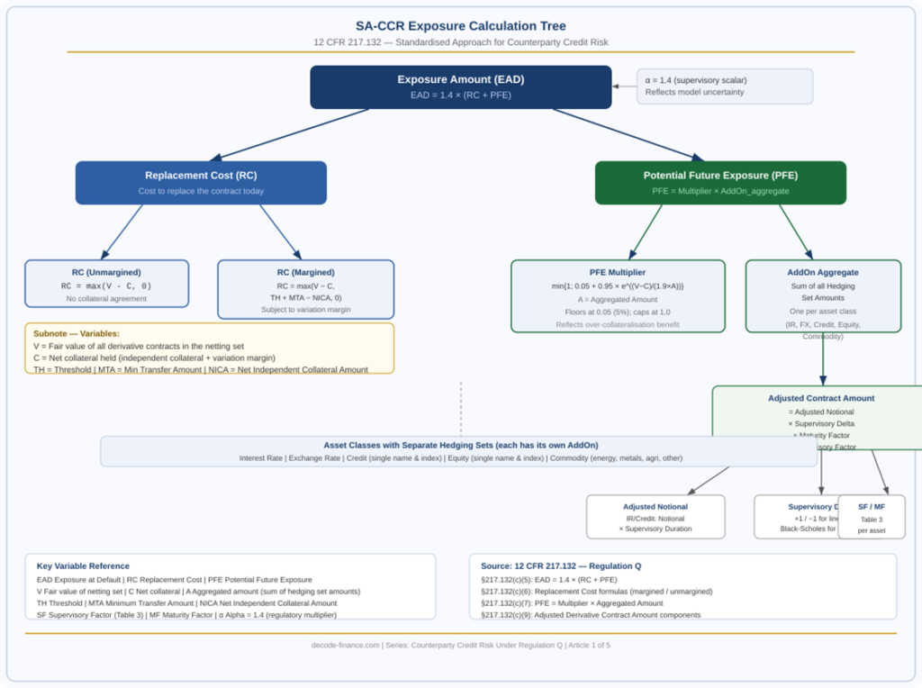
Reading the Diagram
Starting from the top:
- EAD = 1.4 × (RC + PFE). The 1.4 multiplier (alpha) is a regulatory constant that adds a conservative buffer.
- Replacement Cost (RC) splits into two paths depending on whether the netting set is subject to a variation margin agreement. The unmargined RC is simply max(V-C, 0). The margined RC accounts for thresholds and minimum transfer amounts.
- Potential Future Exposure (PFE) is the product of the PFE Multiplier and the Aggregated Amount (the sum of all Hedging Set Amounts across asset classes).
- The PFE Multiplier compresses PFE when collateral exceeds the net fair value — rewarding over-collateralisation. It can never go below 5%.
- Each Hedging Set Amount is built up from Adjusted Derivative Contract Amounts — which are themselves the product of four components: Adjusted Notional, Supervisory Delta, Maturity Factor, and Supervisory Factor.
The Key Variables at a Glance
| Term | Plain English Meaning |
| V | Fair value of all derivative contracts in the netting set (positive means the counterparty owes money to the bank) |
| C | Net collateral held — sum of independent collateral and variation margin, after haircuts |
| TH | Threshold — exposure level below which no collateral call is triggered under the margin agreement |
| MTA | Minimum Transfer Amount — smallest collateral transfer that can be made under the agreement |
| NICA | Net Independent Collateral Amount — initial margin held, net of initial margin posted to the same counterparty |
| A | Aggregated Amount — sum of all Hedging Set Amounts across all asset classes in the netting set |
| SF | Supervisory Factor — asset-class specific scaling factor (e.g., 0.5% for interest rates, 32% for single-name equities) |
| MF | Maturity Factor — adjusts for the remaining life of the contract and the margin period of risk |
| α (alpha) | 1.4 — the regulatory multiplier applied to the sum of RC and PFE. Higher alpha can be imposed by the Board for specific institutions. |
Quick Summary
- Counterparty credit risk is the risk that the other party to a derivative contract defaults before fulfilling their obligations.
- EAD (Exposure at Default) measures the maximum likely loss at the point of default. Under SA-CCR: EAD = 1.4 × (RC + PFE).
- PD (Probability of Default) estimates how likely the counterparty is to default. Higher PD means more capital required.
- LGD (Loss Given Default) estimates the fraction of exposure that cannot be recovered. Together with EAD and PD, it drives expected loss calculations.
- Credit Spreads reflect the market’s assessment of counterparty default risk and are central to CVA calculations.
- Netting allows multiple contracts with the same counterparty to be offset, dramatically reducing gross exposure.
- Collateral reduces both current exposure (in RC) and potential future exposure (via the PFE Multiplier). Haircuts ensure conservative valuation.
Frequently Asked Questions
What is counterparty credit risk in simple terms?
Counterparty credit risk is the risk that the other party to a financial contract — a loan, a derivative, a repo — defaults before fulfilling their payment obligations. Unlike market risk, which arises from price movements, counterparty credit risk arises from the failure of a specific entity.
What is the difference between EAD, PD, and LGD?
EAD is how much is at risk. PD is the probability that the counterparty actually defaults. LGD is what fraction of the exposure is lost if they do default. Together: Expected Loss = EAD × PD × LGD.
Why does SA-CCR use a multiplier of 1.4?
The 1.4 multiplier (alpha) is a regulatory conservatism factor. It reflects empirical evidence that simplified models — which calculate EAD as just Replacement Cost plus Potential Future Exposure — tend to underestimate true exposure. The multiplier builds in a 40% buffer. Banks can apply to the Federal Reserve to use their own alpha estimate, subject to a floor of 1.2.
What is a netting set?
A netting set is a group of derivative contracts between two counterparties that are subject to a legally enforceable netting agreement. Within a netting set, positive and negative fair values can be offset, reducing the exposure to the net position rather than the sum of gross positions.
How does collateral reduce counterparty credit risk?
Collateral reduces EAD directly. In the SA-CCR framework, collateral (C) is subtracted from the fair value of the portfolio (V) when calculating Replacement Cost. Initial margin also reduces the PFE Multiplier, compressing potential future exposure when the portfolio is over-collateralised. All collateral is subject to supervisory haircuts to reflect the risk that collateral values can fall.
What is the difference between variation margin and initial margin? Variation margin is exchanged daily based on changes in the mark-to-market value of the portfolio. It reflects current exposure. Initial margin is posted at the start of a trade as a forward-looking buffer against potential future exposure. Under SA-CCR, initial margin that a bank holds from a counterparty is treated as NICA (Net Independent Collateral Amount) and reduces both Replacement Cost and PFE.
What We Cover in the Remaining 4 Articles
This article has established the foundation. Here is what each subsequent article in this series will cover:
| Term | Topics |
| Part 2 | Replacement Cost in Full — Margined and Unmargined netting sets, haircut methodology, and collateral recognition under §217.132(b) |
| Part 3 | Potential Future Exposure — The PFE Multiplier, Hedging Set Amounts, Adjusted Notional, Supervisory Delta, and Maturity Factor under §217.132(c)(7)–(c)(9) |
| Part 4 | Credit Valuation Adjustment (CVA) — Simple and Advanced CVA approaches, hedging, and stress testing under §217.132(e) |
| Part 5 | Internal Models Methodology — How banks can use their own models for EAD, the approval process, and wrong-way risk under §217.132(d) |